Bollinger Bands with Python applied to the S&P500

Using Bollinger Bands, we can create a trading strategy to buy and sell stocks based on the market’s moving volatility.

We explain the process as we apply the strategy to the S&P500 data.

Data

The S&P500 is an index that represents the performance of the 500 largest companies in the United States.

To simplify understanding, we selected one year of data.

import yfinance as yf
df = yf.download('SPY', start='2023-01-01', end='2024-01-01')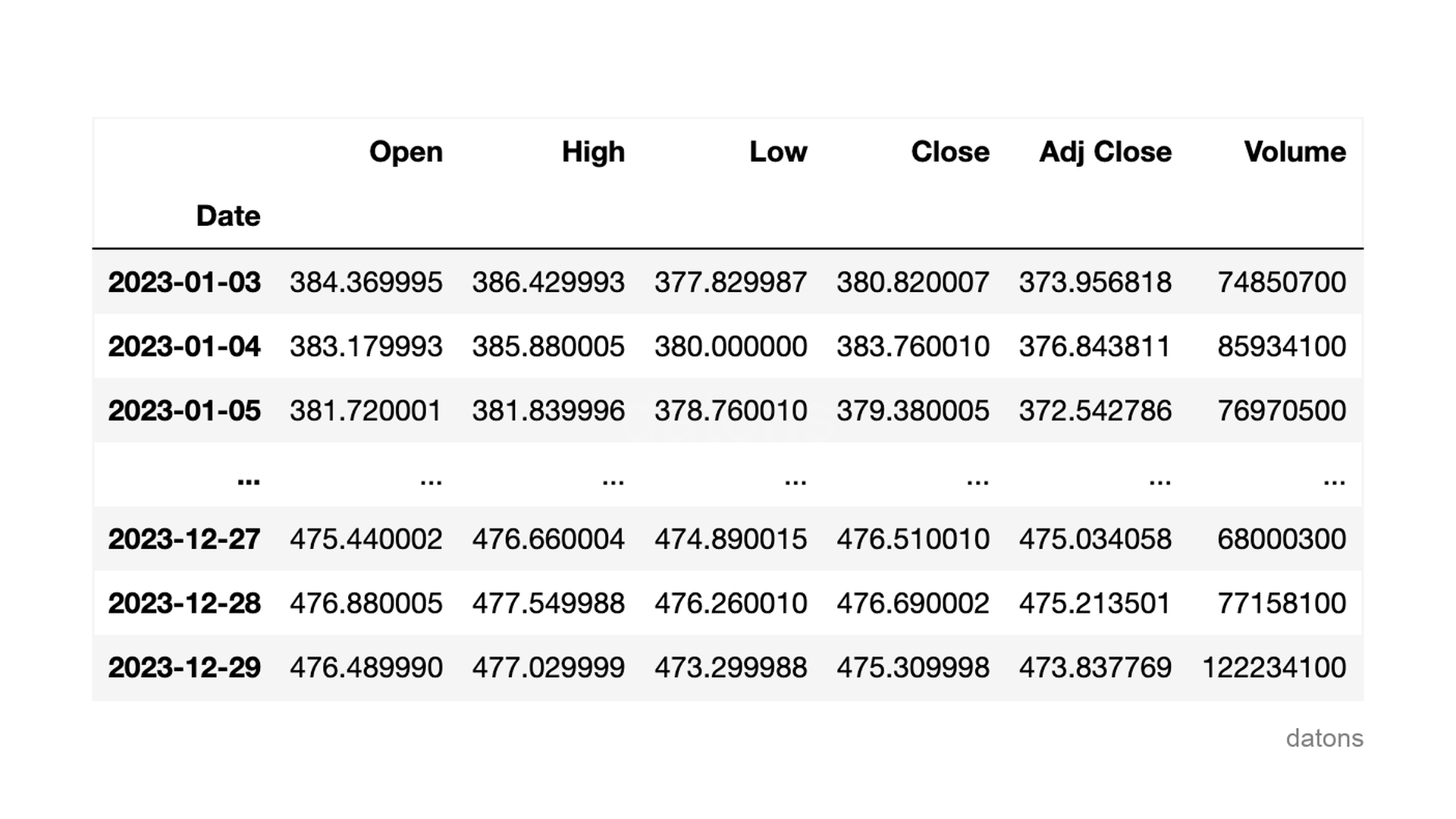

Questions

1. What are Bollinger Bands, and how are they calculated?
2. How to determine buy and sell signals with Bollinger Bands?
3. How to avoid consecutive buy or sell signals in the trading strategy?
4. How to calculate the outcome of the strategy?

Methodology

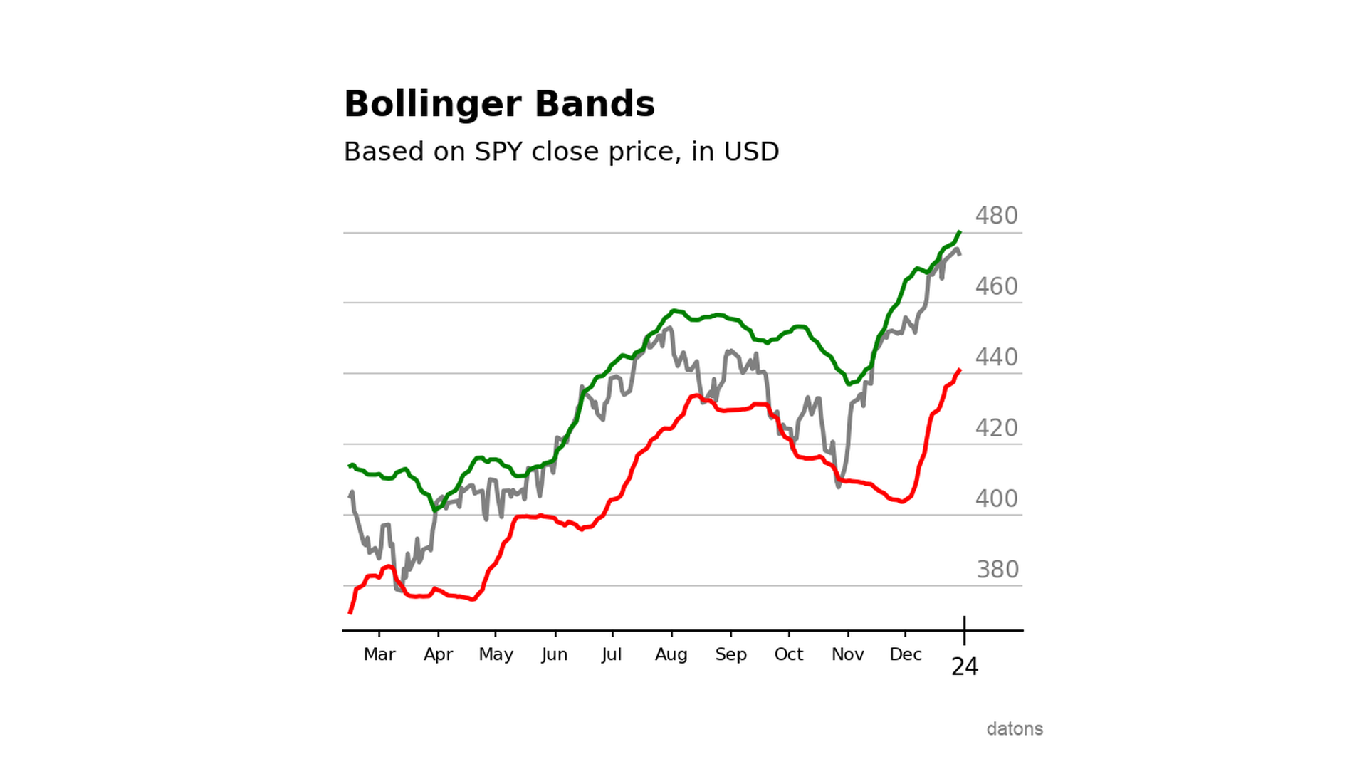
Moving Averages and Standard Deviations

Bollinger Bands are calculated from the moving average (\(\)) and standard deviation (\(\)) based on a period \(r\).

\(\) bands = _r k _r \(\)

In our case, we will use 30 days.

df['Adj Close'].rolling(30).agg(['mean', 'std'])

Calculating Bands

Besides choosing the period, we must select the width of the bands with the \(k\) parameter, which will multiply the standard deviation.

(df
 .assign(
     b_lower = lambda x: x['mean'] - 2 * x['std'],
     b_upper = lambda x: x['mean'] + 2 * x['std']
 )
)

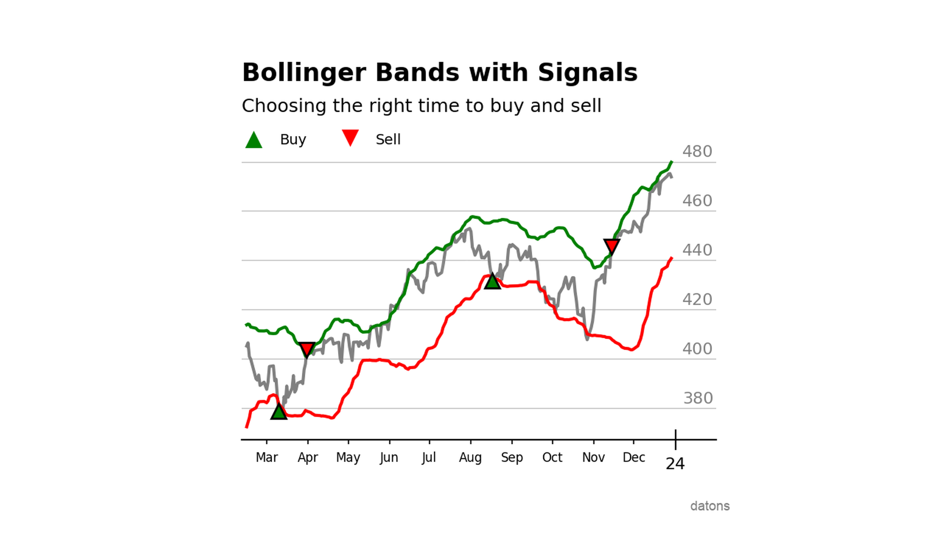
Buy and Sell Signals

Now comes the juiciest (and most complicated) part: calculating the buy and sell points.

If the closing price crosses the lower band, the asset is undervalued (worth more than it costs) and is likely to rise. Therefore, it is a buy signal.

For selling, we will use the crossing of the upper band.

Would this be interesting to one of your friends? Share it with them.

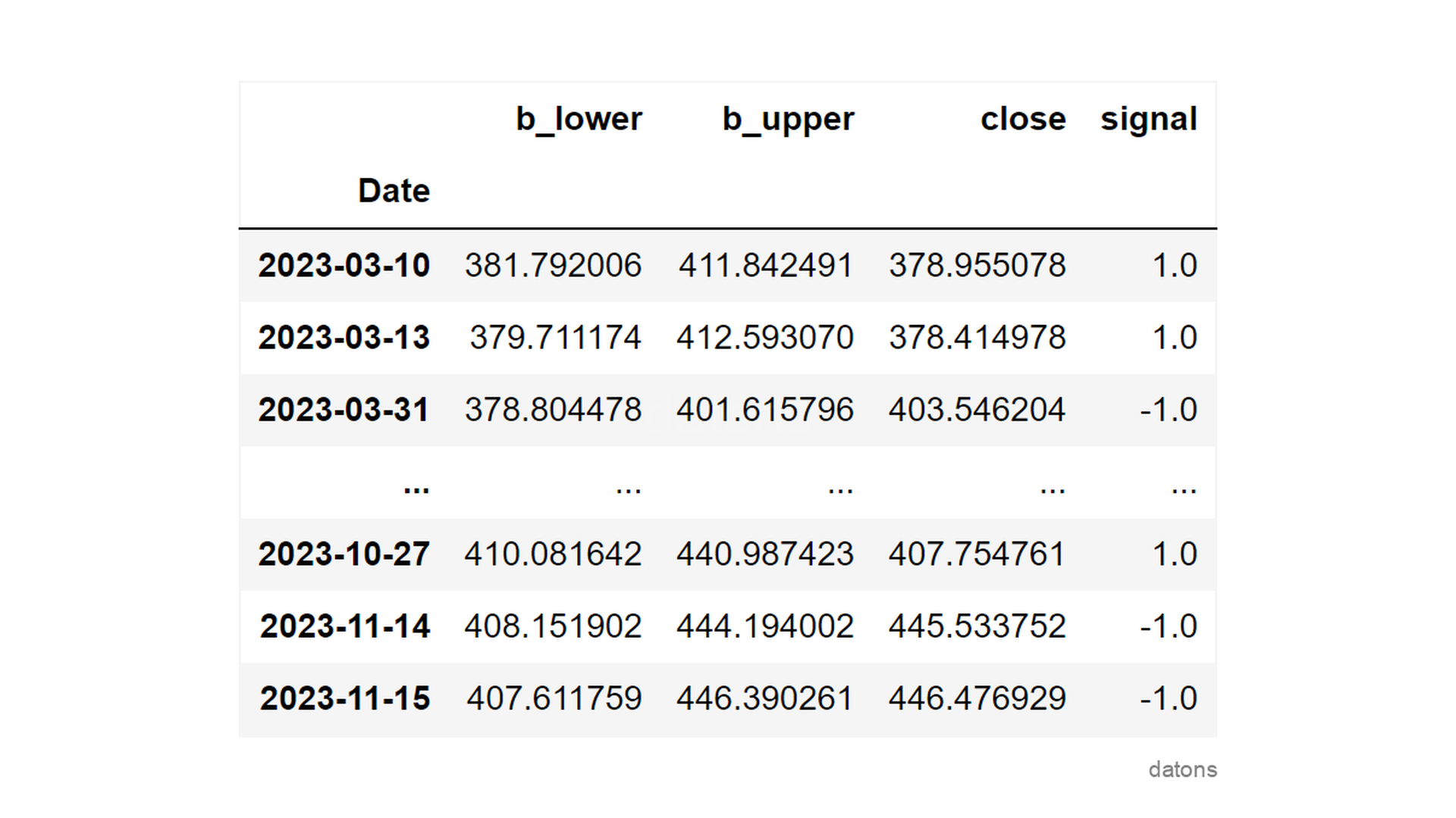
mask_sell = df.close > df.b_upper
mask_buy = df.close < df.b_lower

df.loc[mask_buy, 'signal'] = 1
df.loc[mask_sell, 'signal'] = -1

Here are the days when we should buy and sell.

But, if we invest all the capital in each operation, we cannot buy if we have already bought, nor sell if we have already sold.

There should not be two consecutive buy (1) or sell (-1) signals.

Signal Control

To avoid the above problem, we will consider the current state of operations with a flag. By default, it will be False because we do not have any open operation (we have not bought one).

flag_buy = False

We iterate over each day to calculate the signals according to the previous conditions.

l = []

for idx, day in df.iterrows():
    if (day.signal == 1) & (flag_buy == False):
        signal = 1
        flag_buy = True
    elif (day.signal == -1) & (flag_buy == True):
        signal = -1
        flag_buy = False
    else:
        signal = 0
        
    l.append(signal)
    
df['signal'] = l

And we get the corrected signals, with only one buy or sell signal followed.

Strategy Outcome

Finally, we calculate the outcome of the strategy.

If we always buy with the same amount, the result will be the sum of the differences between the moments of purchase and sale.

(df.close * df.signal).mul(-1).sum()

Therefore, if we had bought one complete share at each signal, we would have obtained a total profit of $38.46 at the end of the period.

Questions? Let’s talk in the comments below.

Conclusions

1. Bollinger Bands: rolling(n).agg(['mean', 'std']) calculates the moving average and standard deviation, the basis for Bollinger Bands, a measure of volatility.
2. Buy/Sell signals: Optimal moments based on Bollinger Bands are identified using the condition df.close < df.b_lower for buying and df.close > df.b_upper for selling.
3. Signal control: By implementing a flag and a loop, consecutive signals of the same type are avoided.
4. Strategy outcome: (df.close * df.signal).mul(-1).sum() sums the differences between the buy and sell points.

If you could program whatever you wanted, what would it be? The upcoming tutorial might cover it ;)

Let’s talk in the comments below.