Working with temporal properties using pandas Datetime Index

The electricity generated by a photovoltaic solar plant varies significantly according to the hour and month.

The energy generation at 18:00 is not the same as at 21:00, nor in January as in June.

Data

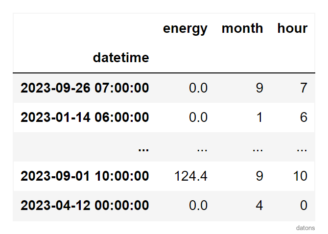
The raw data represent solar energy generation at a photovoltaic plant over the course of the year 2023.

import pandas as pd

df = pd.read_csv('data.csv')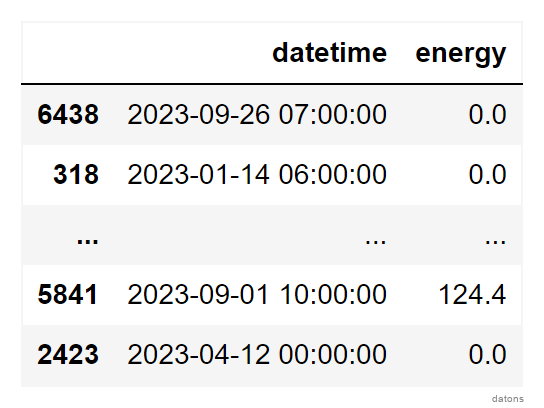

Questions

To create the report from the raw data, we need to answer the following questions:

1. How to format the temporal column with pandas?
2. Why is it useful to set the temporal column as an index?
3. How to create independent temporal columns?
4. How to aggregate data based on hour and month?
5. How to filter data relevant for analysis?
6. What technique highlights the variation in energy generation throughout the day?

Methodology

Formatting Temporal Column

The temporal column must be recognized as a datetime object to work with the temporal properties offered by pandas.

For this, we use the pd.to_datetime function.

df['datetime'] = pd.to_datetime(df['datetime'])
df.dtypes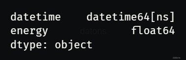

Temporal Column to Index

If our data table has a temporal column with unique values, it’s good practice to set it as an index.

df.set_index('datetime', inplace=True)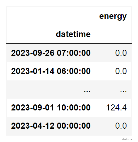

Creating Independent Temporal Columns

We would like to aggregate the total energy generation by month and hour. To do this, we create two new columns: month and hour.

Would this be interesting to one of your friends? Share it with them.

df = (df
 .assign(
     month = df.index.month,
     hour = df.index.hour,
    )
)

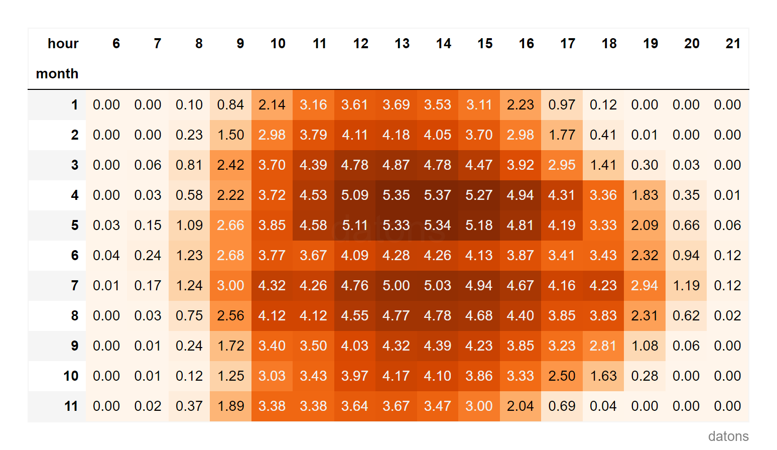
Aggregating Data by Hour and Month

Having new columns that can be interpreted as categorical, we use the pivot_table function to create a report table representing the total energy generation by month and hour.

dfr = (df
 .pivot_table(
     index='month', columns='hour',
     values='energy', aggfunc='sum'
    )
)

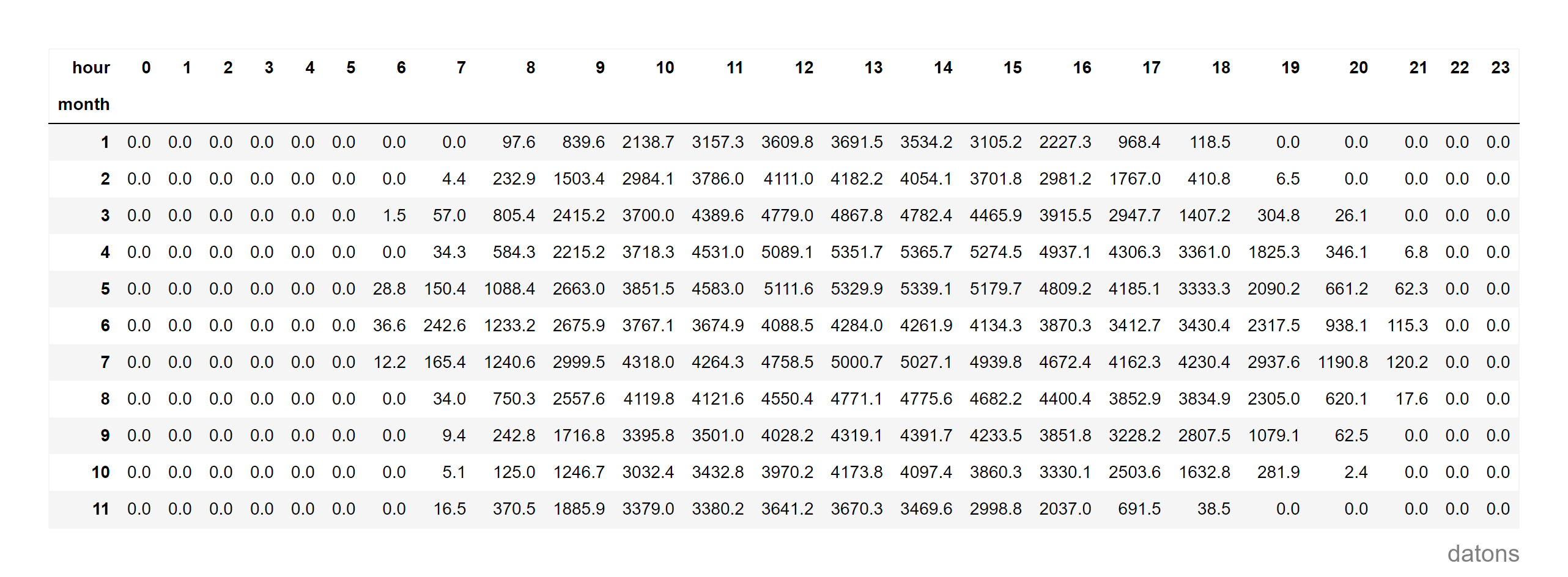
Locating Relevant Data

As expected, solar generation produces 0 energy during the night.

To clean up the table, we select with loc the hours from 6:00 to 21:00.

dfr.loc[:, 6:21]

Heat Matrix Analysis

The report is quite bland; it needs some salt and a bit of spice.

We add it following this recipe et voilà.

It’s curious that, just before the summer starts, in full June, the generation does not continue the trend from spring. What happened?

Looking forward to reading your comments.

Conclusions

In conclusion, thanks to this tutorial we have answered the questions posed at the beginning:

1. Formatting the temporal column: pd.to_datetime converts the specified column to date and time format.
2. Setting the temporal column as an index: set_index facilitates temporal operations by making the time column the DataFrame index.
3. Creating independent temporal columns: DatetimeIndex allows extracting independent temporal properties.
4. Aggregating data based on hour and month: pivot_table organizes data by month and hour, useful for aggregate analysis.
5. Filtering data relevant for analysis: loc selects segments of the DataFrame.
6. Highlighting the variation in energy generation throughout the day: pivot_table combined with color gradients highlights temporal patterns.

If you could program whatever you wanted, what would it be?

I might give you a hand by creating tutorials that help you. I’ll read you in the comments.